External tools
Post-processing for charge density, band density, DOS, STM
The utility PostProcessCQ
allows users to post-process the output
of a CONQUEST calculation, to produce the charge density, band
densities, DOS and STM images in useful forms (at present, as a CUBE
file which can be read by the VESTA code, which is freely available).
There are a number of different analyses which can be performed:
coordinate conversion (to formats which can be plotted); conversion of
total charge density to CUBE file format; production of band-resolved
(optionally k-point resolved) densities in CUBE file format; simple
Tersoff-Hamann STM simulation; and calculation of densities of states
(projected DOS is under development). You should ensure that all the
files produced during the CONQUEST run are available for the
post-processing (including eigenvalues.dat
, chden.nnn
,
make_blk.dat
or hilbert_make_blk.dat
) as well as the input
files.
Note that the utility reads the Conquest_input
file, taking some
flags from the CONQUEST run that generated the output, and some
utility-specific flags that are detailed below.
Note also that band density and STM simulation are not at present compatible with multi-site support functions (MSSF), though we hope to implement this soon.
Go to top.
Coordinate conversion
Set Process.Job coo
to output a coordinate file for further
processing or plotting. The utility will read the file specified by
Process.Coordinates
(which defaults to the file specified by
IO.Coordinates
). The output format is selected by specifying the
Process.CoordFormat
tag. The default output format is XYZ (which
adds a .xyz
suffix to the file name) using xyz
. The CASTEP
.cell output format can also be selected using cell
. We plan to
expand this conversion to other formats in the future.
Note that for a structural relaxation or molecular dynamics
calculation, if you do not specify Process.Coordinates
then the
IO.Coordinates
file, which will be converted, will be the input
structure, not the output structure. Parameters that can be set are:
Process.Coordinates string (default: IO.Coordinates value)
Process.CoordFormat string (default: xyz)
Go to top.
Charge density
Setting Process.Job
to cha
, chg
or den
will convert
the files chden.nnn
which are written by CONQUEST to a cube file.
The processing will use the files chden.nnn
, Conquest_input
and hilbert_make_blk.dat
or raster_make_blk.dat
. Parameters
that can be set include:
Process.ChargeStub string (default: chden)
The ChargeStub simply defines the filename which will be read, and used for output.
Note that to output the chden.nnn
files from CONQUEST, you must
set the flag IO.DumpChargeDensity
to true in the CONQUEST run.
Go to top.
Band density
Setting Process.Job
to ban
produces band densities from wave
function coefficients output by CONQUEST. The CONQUEST run must have
the following tags set:
IO.outputWF T
A set of bands whose coefficients are output are specified either with an energy range (the default is to produce all bands):
IO.WFRangeRelative T/F
IO.min_wf_E real (Ha)
IO.max_wf_E real (Ha)
or with a list of bands:
IO.maxnoWF n
%block WaveFunctionsOut
n entries, each a band number
%endblock
The wavefunction range can be relative to the Fermi level
(IO.WFRangeRelative T
) otherwise it is absolute. Either of these
will produce a file containing all eigenvalues at all k-points
(eigenvalues.dat
) and a series of files containing the
wavefunction expansion coefficients for the selected bands
(ProcessnnnnnnnWF.dat
). From these, band densities can be
produced in post-processing, using similar tags; either a range:
Process.min_wf_E real (Ha)
Process.max_wf_E real (Ha)
Process.WFRangeRelative T/F
or an explicit list of bands:
Process.noWF n
%block WaveFunctionsProcess
n entries, each a band number
%endblock
Note that the bands to be processed must be a subset of the bands
output by CONQUEST. The bands can be output summed over k-points, or
at individual k-points, by setting Process.outputWF_by_kpoint
to
F
or T
respectively.
Go to top.
Tersoff-Hamann STM simulation
Setting Process.Job ter
will use a very simple Tersoff-Hamann
approach to STM simulation, summing over band densities between the
Fermi level and the bias voltage (this is often surprisingly
accurate). The following parameters can be set:
STM.BiasVoltage real (eV)
STM.FermiOffset real (eV)
Process.MinZ real (Bohr)
Process.MaxZ real (Bohr)
Process.RootFile string (default: STM)
The FermiOffset
tag allows the user to shift the Fermi level (to simulate
charging or an external field). The height of the simulation cell
in which the STM image is calculated is set by the MinZ
and
MaxZ
tags, and the filename by the RootFile
tag.
Go to top.
Density of states
Setting Process.Job dos
will produce a total density of states
(DOS) for the system, using the eigenvalues output by CONQUEST. The
following parameters can be set:
Process.min_DOS_E real (Ha, default lowest eigenvalue)
Process.max_DOS_E real (Ha, default highest eigenvalue)
Process.sigma_DOS real (Ha, default 0.001)
Process.n_DOS integer (default 201)
The limits for the DOS are set by the first two parameters (note that
CONQUEST will output all eigenvalues, so the limits on these are set
by the eigenspectrum). The broadening applied to each state is set by
sigma_DOS
, while the number of bins is set by n_DOS
. The
integrated DOS are also calculated; the user can choose whether this
is the total integrated DOS (i.e. from the lowest eigenvalue,
regardless of the lower limit for DOS) or just the local integrated
DOS (i.e. over the interval specified for the DOS) by setting
Process.TotalIntegratedDOS
to T
or F
, respectively.
We recommend that, for accurate DOS, CONQUEST should be
run non-self-consistently with a very high k-point density, using a
well-converged input charge density: set minE.SelfConsistent F
and
General.LoadRho T
.
Atom-projected DOS will be available soon.
Go to top.
Molecular dynamics analysis
Several scripts that may be helpful with postprocessing molecular dynamics are
included with CONQUEST. The can be found in the tools
directory, and the
executables are plot_stats.py
, md_analysis.py
and heat_flux.py
. They
have the following dependencies:
Python 3
Scipy/Numpy
Matplotlib
If Python 3 is installed the modules can be added easily using pip3 install
scipy
etc.
These scripts should be run in the calculation directory, and will automatically
parse the necessary files, namely Conquest_input
, input.log
,
md.stats
and md.frames
assuming they have the default names. They will
also read the CONQUEST input flags to determine, for example, what ensemble is
used, and process the results accordingly.
Go to top.
Plotting statistics
usage: plot_stats.py [-h] [-c] [-d DIRS [DIRS ...]]
[--description DESC [DESC ...]] [--skip NSKIP]
[--stop NSTOP] [--equil NEQUIL] [--landscape]
[--mser MSER_VAR]
Plot statistics for a CONQUEST MD trajectory
optional arguments:
-h, --help show this help message and exit
-c, --compare Compare statistics of trajectories in directories
specified by -d (default: False)
-d DIRS [DIRS ...], --dirs DIRS [DIRS ...]
Directories to compare (default: .)
--description DESC [DESC ...]
Description of graph for legend (only if using
--compare) (default: )
--skip NSKIP Number of equilibration steps to skip (default: 0)
--stop NSTOP Number of last frame in analysis (default: -1)
--equil NEQUIL Number of equilibration steps (default: 0)
--landscape Generate plot with landscape orientation (default:
False)
--mser MSER_VAR Compute MSER for the given property (default: None)
Running plot_stats.py --skip 200
in your calculation will generate a plot
which should resemble the example below, skipping the first 200 steps. This
example is a molecular dynamics simulation of 1000 atoms of bulk silicon in the
NPT ensemble, at 300 K and 0.1 GPa.

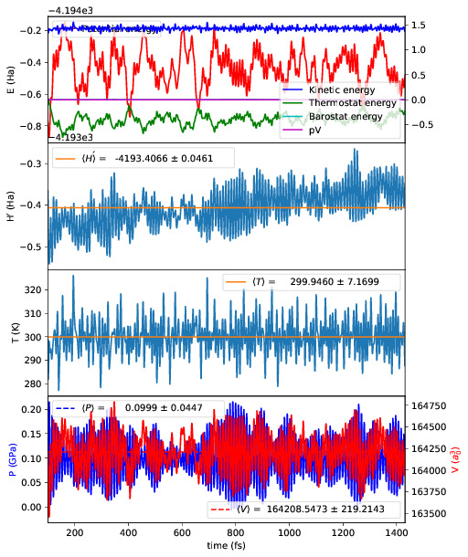
The four plots are respectively the breakdown of energy contributions, the
conserved quantity, the temperature and the pressure, the last of which is only
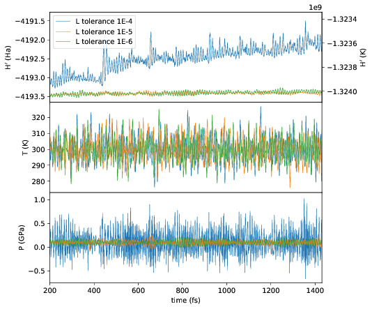
included for NPT molecular dynamics. Several calculations in different
directories can be compared using plot_stats.py --compare -d dir1
dir2 --description "dir1 description" "dir2 description"
. The following
example compares the effect of changing the L tolerance in the above simulation.
Note that the contents of the description field will be in the legend of the
plot.

Go to top.
MD analysis
usage: md_analysis.py [-h] [-d DIRS [DIRS ...]] [--skip NSKIP]
[--stride STRIDE] [--snap SNAP] [--stop NSTOP]
[--equil NEQUIL] [--vacf] [--msd] [--rdf] [--stress]
[--nbins NBINS] [--rdfwidth RDFWIDTH] [--rdfcut RDFCUT]
[--window WINDOW] [--fitstart FITSTART] [--dump]
Analyse a CONQUEST MD trajectory
optional arguments:
-h, --help show this help message and exit
-d DIRS [DIRS ...], --dirs DIRS [DIRS ...]
Directories to compare (default: .)
--skip NSKIP Number of equilibration steps to skip (default: 0)
--stride STRIDE Only analyse every nth step of frames file (default:
1)
--snap SNAP Analyse Frame of a single snapshot (default: -1)
--stop NSTOP Number of last frame in analysis (default: -1)
--equil NEQUIL Number of equilibration steps (default: 0)
--vacf Plot velocity autocorrelation function (default:
False)
--msd Plot mean squared deviation (default: False)
--rdf Plot radial distribution function (default: False)
--stress Plot stress (default: False)
--nbins NBINS Number of histogram bins (default: 100)
--rdfwidth RDFWIDTH RDF histogram bin width (A) (default: 0.05)
--rdfcut RDFCUT Distance cutoff for RDF in Angstrom (default: 8.0)
--window WINDOW Window for autocorrelation functions in fs (default:
1000.0)
--fitstart FITSTART Start time for curve fit (default: -1.0)
--dump Dump secondary data used to generate plots (default:
False)
The script md_analysis.py
script performs various analyses of the trajectory
by parsing the md.frames` file. So far, these include the radial distribution
function, the velocity autocorrelation function, the mean squared deviation, and
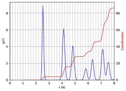
plotting the stress. For example, the command,
md_analysis.py --rdf --stride 20 --rdfcut 8.0 --nbins 100 --dump --skip 200 --stop 400
computes the radial distribution function of the simulation in the first example from every 20th time step (every 10 fs in this case), stopping after 400 steps, with a cutoff of 8.0 A, and the histogram is divided into 100 bins.

Go to top.
CONQUEST structure file analysis
usage: structure.py [-h] [-i INFILE] [--bonds] [--density] [--nbins NBINS]
[-c CUTOFF [CUTOFF ...]] [--printall]
Analyse a CONQUEST-formatted structure
optional arguments:
-h, --help show this help message and exit
-i INFILE, --infile INFILE
CONQUEST format structure file (default:
coord_next.dat)
--bonds Compute average and minimum bond lengths (default:
False)
--density Compute density (default: False)
--nbins NBINS Number of histogram bins (default: 100)
-c CUTOFF [CUTOFF ...], --cutoff CUTOFF [CUTOFF ...]
Bond length cutoff matrix (upper triangular part, in
rows (default: None)
--printall Print all bond lengths (default: False)
The script structure.py
can be used to analyse a CONQUEST-formatted
structure file. This is useful to sanity-check the bond lengths or density,
since an unphysical structure is so often the cause of a crash. For example, the
bond lengths can be computed with
structure.py --bonds -c 2.0 3.0 3.0
where the -c
flag specifies the bond cutoffs for the bonds 1-1, 1-2 and 2-2,
where 1 is species 1 as specified in Conquest_input
and 2 is species 2. The
output will look something like this:
Mean bond lengths:
O-Si: 1.6535 +/- 0.0041 (24 bonds)
Minimum bond lengths:
O-Si: 1.6493
Go to top.
Atomic Simulation Environment (ASE)
ASE is a set of Python tools for setting up, manipulating, running, visualizing and analyzing atomistic simulations. ASE contains a CONQUEST interface, so that it can be used to calculate energies, forces and stresses for calculations that CONQUEST can’t do (yet). Detailed instructions on how to install and invoke it can be found on its website, but we provide some details and examples for the CONQUEST interface here.
Note that the script will need to set environmental variables specifying the
locations of the CONQUEST executable Conquest
, and if required, the basis
set generation executable MakeIonFiles
and pseudopotential database.
import os
# The command to run CONQUEST in parallel
os.environ["ASE_CONQUEST_COMMAND"] = "mpirun -np 4 /path/to/Conquest_master"
# Path to a database of pseudopotentials (for basis generation tool)
os.environ["CQ_PP_PATH"] = "~/Conquest/PPDB/"
# Path to the basis generation tool executable
os.environ["CQ_GEN_BASIS_CMD"] = "/path/to/MakeIonFiles"
Go to top.
Keywords for generating the Conquest_input file
The calculator object contains a dictionray containing a small number of mandatory keywords, listed below:
default_parameters = {
'grid_cutoff' : 100, # DFT defaults
'kpts' : None,
'xc' : 'PBE',
'scf_tolerance' : 1.0e-6,
'nspin' : 1,
'general.pseudopotentialtype' : 'Hamann', # CONQUEST defaults
'basis.basisset' : 'PAOs',
'io.iprint' : 2,
'io.fractionalatomiccoords' : True,
'mine.selfconsistent' : True,
'sc.maxiters' : 50,
'atommove.typeofrun' : 'static',
'dm.solutionmethod' : 'diagon'}
The first five key/value pairs are special DFT parameters, the grid cutoff, the k-point mesh, the exchange-correlation functional, the SCF tolerance and the number of spins respectively. The rest are CONQUEST-specific input flags.
The atomic species blocks are handled slightly differently, with a dictionary of
their own. If the .ion
files are present in the calculation directory, they
can be specified as follows:
basis = {"H": {"valence_charge": 1.0,
"number_of_supports": 1,
"support_fn_range": 6.9},
"O": {"valence_charge": 6.0,
"number_of_supports": 4,
"support_fn_range": 6.9}}
If the basis set .ion
files are present in the directory containing the ASE
script are pressent and are named element.ion
, then the relevant parameters
will be parsed from the .ion
files and included when the input file is
written and this dictionary can be omitted. It is more important when, for
example, setting up a multisite calculation, when the number of contracted
support functions is different from the number in the .ion
file.
ASE can also invoke the CONQUEST basis set generation tool, although care should be taken when generating basis sets:
basis = {"H": {"basis_size": "minimal",
"pseudopotential_type": hamann",
"gen_basis": True},
"O": {"basis_size": "minimal",
"pseudopotential_type": hamann",
"gen_basis": True}}
Finally, non-mandatory input flags can be defined in a new dictionary, and passed as an expanded set of keyword arguments.
conquest_flags = {'IO.Iprint' : 1, # CONQUEST keywords
'DM.SolutionMethod' : 'ordern',
'DM.L_range' : 8.0,
'minE.LTolerance' : 1.0e-6}
Here is an example, combining the above. We set up a cubic diamond cell containing 8 atoms, and perform a single point energy calculation using the order(N) method (the default is diagonalisation, so we must specify all of the order(N) flags). We don’t define a basis set, instead providing keywords that specify that a minimal basis set should be constructed using the MakeIonFiles basis generation tool.
from ase.build import bulk
from ase.calculators.conquest import Conquest
os.environ["ASE_CONQUEST_COMMAND"] = "mpirun -np 4 Conquest_master"
os.environ["CQ_PP_PATH"] = "/Users/zamaan/Conquest/PPDB/"
os.environ["CQ_GEN_BASIS_CMD"] = "MakeIonFiles"
diamond = bulk('C', 'diamond', a=3.6, cubic=True) # The atoms object
conquest_flags = {'IO.Iprint' : 1, # Conquest keywords
'DM.SolutionMethod' : 'ordern',
'DM.L_range' : 8.0,
'minE.LTolerance' : 1.0e-6}
basis = {'C': {"basis_size" : 'minimal', # Generate a minimal basis
"gen_basis" : True,
"pseudopotential_type" : "hamann"}}
calc = Conquest(grid_cutoff = 80, # Set the calculator keywords
xc="LDA",
self_consistent=True,
basis=basis,
nspin=1,
**conquest_flags)
diamond.set_calculator(calc) # attach the calculator to the atoms object
energy = diamond.get_potential_energy() # calculate the potential energy
Go to top.
Multisite support functions
Multisite support functions require a few additional keywords in the atomic species block, which can be specified as follows:
basis = {'C': {"basis_size": 'medium',
"gen_basis": True,
"pseudopotential_type": "hamann",
"Atom.NumberofSupports": 4,
"Atom.MultisiteRange": 7.0,
"Atom.LFDRange": 7.0}}
Note that we are constructing a DZP basis set (size medium) with 13 primitive
support functions using MakeIonFiles
, and contracting it to multisite basis
of 4 support functions. The calculation requires a few more input flags, which
are specified in the other_keywords
dictionary:
other_keywords = {"Basis.MultisiteSF": True,
"Multisite.LFD": True,
"Multisite.LFD.Min.ThreshE": 1.0e-7,
"Multisite.LFD.Min.ThreshD": 1.0e-7,
"Multisite.LFD.Min.MaxIteration": 150,
}
Go to top.
Loading the K/L matrix
Most calculation that involve incrementally moving atoms (molecular dynamics, geometry optimisation, equations of state, nudged elastic band etc.) can be made faster by using the K or L matrix from a previous calculation as the initial guess for a subsequent calculation in which that atoms have been moved slightly. This can be achieved by first performing a single point calculation to generate the first K/L matrix, then adding the following keywords to the calculator:
other_keywords = {"General.LoadL": True,
"SC.MakeInitialChargeFromK": True}
These keywords respectively cause the K or L matrix to be loaded from file(s)
Kmatrix.i**.p*****
, and the initial charge density to be constructed from
this matrix. In all subsequent calculations, the K or L matrix will be written
at the end of the calculation and used as the initial guess for the subsequent
ionic step.
Go to top.
Equation of state
The following code computes the equation of state of diamond by doing single
point calculations on a uniform grid of the a
lattice parameter. It then
interpolates the equation of state and uses matplotlib
to generate a plot.
import scipy as sp
from ase.build import bulk
from ase.io.trajectory import Trajectory
from ase.calculators.conquest import Conquest
# Construct a unit cell
diamond = bulk('C', 'diamond', a=3.6, cubic=True)
basis = {'C': {"basis_size": 'minimal',
"gen_basis": True,
"pseudopotential_type": "hamann"}}
calc = Conquest(grid_cutoff = 50,
xc = "LDA",
basis = basis,
kpts = [4,4,4]}
diamond.set_calculator(calc)
cell = diamond.get_cell()
traj = Trajectory('diamond.traj', 'w') # save all results to trajectory
for x in sp.linspace(0.95, 1.05, 5): # grid for equation of state
diamond.set_cell(cell*x, scale_atoms=True)
diamond.get_potential_energy()
traj.write(diamond)
from ase.io import read
from ase.eos import EquationOfState
configs = read('diamond.traj@0:5')
volumes = [diamond.get_volume() for diamond in configs]
energies = [diamond.get_potential_energy() for diamond in configs]
eos = EquationOfState(volumes, energies)
v0, e0, B = eos.fit()
import matplotlib
eos.plot('diamond-eos.pdf') # Plot the equation of state
Go to top.