External tools
Molecular dynamics analysis
Several scripts that may be helpful with postprocessing molecular dynamics are
included with CONQUEST. The can be found in the tools directory, and the
executables are plot_stats.py, md_analysis.py and heat_flux.py. They
have the following dependencies:
Python 3
Scipy/Numpy
Matplotlib
If Python 3 is installed the modules can be added easily using pip3 install
scipy etc.
These scripts should be run in the calculation directory, and will automatically
parse the necessary files, namely Conquest_input, input.log,
md.stats and md.frames assuming they have the default names. They will
also read the CONQUEST input flags to determine, for example, what ensemble is
used, and process the results accordingly.
Go to top.
Plotting statistics
usage: plot_stats.py [-h] [-c] [-d DIRS [DIRS ...]]
                    [--description DESC [DESC ...]] [--skip NSKIP]
                    [--stop NSTOP] [--equil NEQUIL] [--landscape]
                    [--mser MSER_VAR]

Plot statistics for a CONQUEST MD trajectory

optional arguments:
  -h, --help            show this help message and exit
  -c, --compare         Compare statistics of trajectories in directories
                        specified by -d (default: False)
  -d DIRS [DIRS ...], --dirs DIRS [DIRS ...]
                        Directories to compare (default: .)
  --description DESC [DESC ...]
                        Description of graph for legend (only if using
                        --compare) (default: )
  --skip NSKIP          Number of equilibration steps to skip (default: 0)
  --stop NSTOP          Number of last frame in analysis (default: -1)
  --equil NEQUIL        Number of equilibration steps (default: 0)
  --landscape           Generate plot with landscape orientation (default:
                        False)
  --mser MSER_VAR       Compute MSER for the given property (default: None)
Running plot_stats.py --skip 200 in your calculation will generate a plot
which should resemble the example below, skipping the first 200 steps. This
example is a molecular dynamics simulation of 1000 atoms of bulk silicon in the
NPT ensemble, at 300 K and 0.1 GPa.
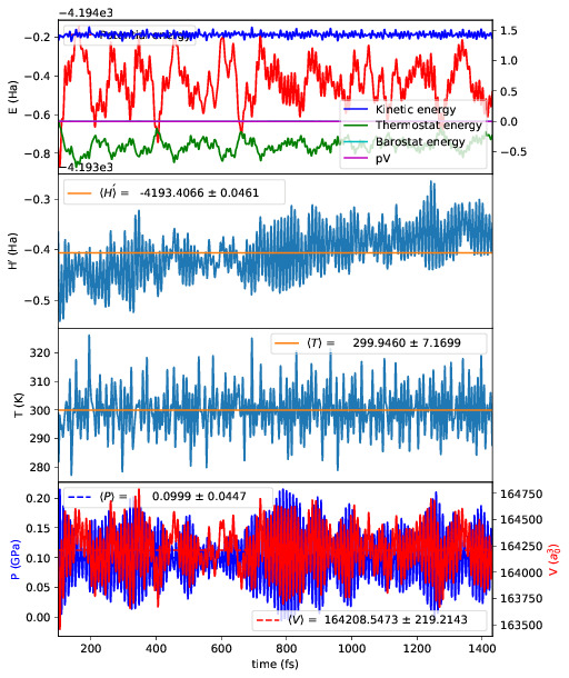
The four plots are respectively the breakdown of energy contributions, the
conserved quantity, the temperature and the pressure, the last of which is only
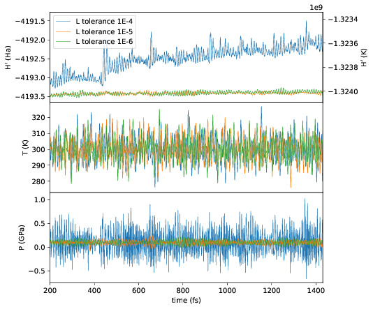
included for NPT molecular dynamics. Several calculations in different
directories can be compared using plot_stats.py --compare -d dir1
dir2 --description "dir1 description" "dir2 description". The following
example compares the effect of changing the L tolerance in the above simulation.
Note that the contents of the description field will be in the legend of the
plot.
Go to top.
MD analysis
usage: md_analysis.py [-h] [-d DIRS [DIRS ...]] [--skip NSKIP]
                      [--stride STRIDE] [--snap SNAP] [--stop NSTOP]
                      [--equil NEQUIL] [--vacf] [--msd] [--rdf] [--stress]
                      [--nbins NBINS] [--rdfwidth RDFWIDTH] [--rdfcut RDFCUT]
                      [--window WINDOW] [--fitstart FITSTART] [--dump]

Analyse a CONQUEST MD trajectory

optional arguments:
  -h, --help            show this help message and exit
  -d DIRS [DIRS ...], --dirs DIRS [DIRS ...]
                        Directories to compare (default: .)
  --skip NSKIP          Number of equilibration steps to skip (default: 0)
  --stride STRIDE       Only analyse every nth step of frames file (default:
                        1)
  --snap SNAP           Analyse Frame of a single snapshot (default: -1)
  --stop NSTOP          Number of last frame in analysis (default: -1)
  --equil NEQUIL        Number of equilibration steps (default: 0)
  --vacf                Plot velocity autocorrelation function (default:
                        False)
  --msd                 Plot mean squared deviation (default: False)
  --rdf                 Plot radial distribution function (default: False)
  --stress              Plot stress (default: False)
  --nbins NBINS         Number of histogram bins (default: 100)
  --rdfwidth RDFWIDTH   RDF histogram bin width (A) (default: 0.05)
  --rdfcut RDFCUT       Distance cutoff for RDF in Angstrom (default: 8.0)
  --window WINDOW       Window for autocorrelation functions in fs (default:
                        1000.0)
  --fitstart FITSTART   Start time for curve fit (default: -1.0)
  --dump                Dump secondary data used to generate plots (default:
                        False)
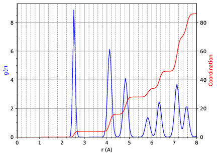
The script md_analysis.py script performs various analyses of the trajectory
by parsing the md.frames` file. So far, these include the radial distribution
function, the velocity autocorrelation function, the mean squared deviation, and
plotting the stress. For example, the command,
md_analysis.py --rdf --stride 20 --rdfcut 8.0 --nbins 100 --dump --skip 200 --stop 400
computes the radial distribution function of the simulation in the first example from every 20th time step (every 10 fs in this case), stopping after 400 steps, with a cutoff of 8.0 A, and the histogram is divided into 100 bins.
Go to top.
CONQUEST structure file analysis
usage: structure.py [-h] [-i INFILE] [--bonds] [--density] [--nbins NBINS]
                    [-c CUTOFF [CUTOFF ...]] [--printall]

Analyse a CONQUEST-formatted structure

optional arguments:
  -h, --help            show this help message and exit
  -i INFILE, --infile INFILE
                        CONQUEST format structure file (default:
                        coord_next.dat)
  --bonds               Compute average and minimum bond lengths (default:
                        False)
  --density             Compute density (default: False)
  --nbins NBINS         Number of histogram bins (default: 100)
  -c CUTOFF [CUTOFF ...], --cutoff CUTOFF [CUTOFF ...]
                        Bond length cutoff matrix (upper triangular part, in
                        rows (default: None)
  --printall            Print all bond lengths (default: False)
The script structure.py can be used to analyse a CONQUEST-formatted
structure file. This is useful to sanity-check the bond lengths or density,
since an unphysical structure is so often the cause of a crash. For example, the
bond lengths can be computed with
structure.py --bonds -c 2.0 3.0 3.0
where the -c flag specifies the bond cutoffs for the bonds 1-1, 1-2 and 2-2,
where 1 is species 1 as specified in Conquest_input and 2 is species 2. The
output will look something like this:
Mean bond lengths:
O-Si:   1.6535 +/-   0.0041 (24 bonds)
Minimum bond lengths:
O-Si:   1.6493
Go to top.
Atomic Simulation Environment (ASE)
ASE is a set of Python tools for setting up, manipulating, running, visualizing and analyzing atomistic simulations. ASE contains a CONQUEST interface, so that it can be used to calculate energies, forces and stresses for calculations that CONQUEST can’t do (yet). Detailed instructions on how to install and invoke it can be found on its website, but we provide some details and examples for the CONQUEST interface here.
Note that the script will need to set environmental variables specifying the
locations of the CONQUEST executable Conquest, and if required, the basis
set generation executable MakeIonFiles and pseudopotential database.
import os

# The command to run CONQUEST in parallel
os.environ["ASE_CONQUEST_COMMAND"] = "mpirun -np 4 /path/to/Conquest_master"
# Path to a database of pseudopotentials (for basis generation tool)
os.environ["CQ_PP_PATH"] = "~/Conquest/PPDB/"
# Path to the basis generation tool executable
os.environ["CQ_GEN_BASIS_CMD"] = "/path/to/MakeIonFiles"
Go to top.
Keywords for generating the Conquest_input file
The calculator object contains a dictionray containing a small number of mandatory keywords, listed below:
default_parameters = {
    'grid_cutoff'   : 100,     # DFT defaults
    'kpts'          : None,
    'xc'            : 'PBE',
    'scf_tolerance' : 1.0e-6,
    'nspin'         : 1,
    'general.pseudopotentialtype' : 'Hamann', # CONQUEST defaults
    'basis.basisset'              : 'PAOs',
    'io.iprint'                   : 2,
    'io.fractionalatomiccoords'   : True,
    'mine.selfconsistent'         : True,
    'sc.maxiters'                 : 50,
    'atommove.typeofrun'          : 'static',
    'dm.solutionmethod'           : 'diagon'}
The first five key/value pairs are special DFT parameters, the grid cutoff, the k-point mesh, the exchange-correlation functional, the SCF tolerance and the number of spins respectively. The rest are CONQUEST-specific input flags.
The atomic species blocks are handled slightly differently, with a dictionary of
their own. If the .ion files are present in the calculation directory, they
can be specified as follows:
basis = {"H": {"valence_charge": 1.0,
               "number_of_supports": 1,
               "support_fn_range": 6.9},
         "O": {"valence_charge": 6.0,
               "number_of_supports": 4,
               "support_fn_range": 6.9}}
If the basis set .ion files are present in the directory containing the ASE
script are pressent and are named element.ion, then the relevant parameters
will be parsed from the .ion files and included when the input file is
written and this dictionary can be omitted. It is more important when, for
example, setting up a multisite calculation, when the number of contracted
support functions is different from the number in the .ion file.
ASE can also invoke the CONQUEST basis set generation tool, although care should be taken when generating basis sets:
basis = {"H": {"basis_size": "minimal",
               "pseudopotential_type": hamann",
               "gen_basis": True},
         "O": {"basis_size": "minimal",
               "pseudopotential_type": hamann",
               "gen_basis": True}}
Finally, non-mandatory input flags can be defined in a new dictionary, and passed as an expanded set of keyword arguments.
conquest_flags = {'IO.Iprint'         : 1,         # CONQUEST keywords
                  'DM.SolutionMethod' : 'ordern',
                  'DM.L_range'        : 8.0,
                  'minE.LTolerance'   : 1.0e-6}
Here is an example, combining the above. We set up a cubic diamond cell containing 8 atoms, and perform a single point energy calculation using the order(N) method (the default is diagonalisation, so we must specify all of the order(N) flags). We don’t define a basis set, instead providing keywords that specify that a minimal basis set should be constructed using the MakeIonFiles basis generation tool.
from ase.build import bulk
from ase.calculators.conquest import Conquest

os.environ["ASE_CONQUEST_COMMAND"] = "mpirun -np 4 Conquest_master"
os.environ["CQ_PP_PATH"] = "/Users/zamaan/Conquest/PPDB/"
os.environ["CQ_GEN_BASIS_CMD"] = "MakeIonFiles"

diamond = bulk('C', 'diamond', a=3.6, cubic=True)  # The atoms object
conquest_flags = {'IO.Iprint'         : 1,         # Conquest keywords
                  'DM.SolutionMethod' : 'ordern',
                  'DM.L_range'        : 8.0,
                  'minE.LTolerance'   : 1.0e-6}
basis = {'C': {"basis_size"           : 'minimal', # Generate a minimal basis
              "gen_basis"             : True,
              "pseudopotential_type"  : "hamann"}}

calc = Conquest(grid_cutoff = 80,    # Set the calculator keywords
                xc="LDA",
                self_consistent=True,
                basis=basis,
                nspin=1,
                **conquest_flags)
diamond.set_calculator(calc)             # attach the calculator to the atoms object
energy = diamond.get_potential_energy()  # calculate the potential energy
Go to top.
Multisite support functions
Multisite support functions require a few additional keywords in the atomic species block, which can be specified as follows:
basis = {'C': {"basis_size": 'medium',
               "gen_basis": True,
               "pseudopotential_type": "hamann",
               "Atom.NumberofSupports": 4,
               "Atom.MultisiteRange": 7.0,
               "Atom.LFDRange": 7.0}}
Note that we are constructing a DZP basis set (size medium) with 13 primitive
support functions using MakeIonFiles, and contracting it to multisite basis
of 4 support functions. The calculation requires a few more input flags, which
are specified in the other_keywords dictionary:
other_keywords = {"Basis.MultisiteSF": True,
                  "Multisite.LFD": True,
                  "Multisite.LFD.Min.ThreshE": 1.0e-7,
                  "Multisite.LFD.Min.ThreshD": 1.0e-7,
                  "Multisite.LFD.Min.MaxIteration": 150,
                  }
Go to top.
Loading the K/L matrix
Most calculation that involve incrementally moving atoms (molecular dynamics, geometry optimisation, equations of state, nudged elastic band etc.) can be made faster by using the K or L matrix from a previous calculation as the initial guess for a subsequent calculation in which that atoms have been moved slightly. This can be achieved by first performing a single point calculation to generate the first K/L matrix, then adding the following keywords to the calculator:
other_keywords = {"General.LoadL": True,
                  "SC.MakeInitialChargeFromK": True}
These keywords respectively cause the K or L matrix to be loaded from file(s)
Kmatrix.i**.p*****, and the initial charge density to be constructed from
this matrix. In all subsequent calculations, the K or L matrix will be written
at the end of the calculation and used as the initial guess for the subsequent
ionic step.
Go to top.
Equation of state
The following code computes the equation of state of diamond by doing single
point calculations on a uniform grid of the a lattice parameter. It then
interpolates the equation of state and uses matplotlib to generate a plot.
import scipy as sp
from ase.build import bulk
from ase.io.trajectory import Trajectory
from ase.calculators.conquest import Conquest


# Construct a unit cell
diamond = bulk('C', 'diamond', a=3.6, cubic=True)

basis = {'C': {"basis_size": 'minimal',
               "gen_basis": True,
               "pseudopotential_type": "hamann"}}
calc = Conquest(grid_cutoff = 50,
                xc = "LDA",
                basis = basis,
                kpts = [4,4,4]}
diamond.set_calculator(calc)

cell = diamond.get_cell()
traj = Trajectory('diamond.traj', 'w') # save all results to trajectory

for x in sp.linspace(0.95, 1.05, 5):   # grid for equation of state
  diamond.set_cell(cell*x, scale_atoms=True)
  diamond.get_potential_energy()
  traj.write(diamond)

from ase.io import read
from ase.eos import EquationOfState

configs = read('diamond.traj@0:5')
volumes = [diamond.get_volume() for diamond in configs]
energies = [diamond.get_potential_energy() for diamond in configs]
eos = EquationOfState(volumes, energies)
v0, e0, B = eos.fit()

import matplotlib
eos.plot('diamond-eos.pdf')    # Plot the equation of state
Go to top.