Example calculations
All example calculations here use diagonalisation and PAO basis sets (with a simple one-to-one mapping between PAOs and support functions).
Static calculation
We will perform a self-consistent electronic structure calculation on bulk silicon. The coordinate file that is needed is:
10.36  0.00  0.00
 0.00 10.36  0.00
 0.00  0.00 10.36
8
  0.000 0.000 0.000  1 T T T
  0.500 0.500 0.000  1 T T T
  0.500 0.000 0.500  1 T T T
  0.000 0.500 0.500  1 T T T
  0.250 0.250 0.250  1 T T T
  0.750 0.750 0.250  1 T T T
  0.250 0.750 0.750  1 T T T
  0.750 0.250 0.750  1 T T T
You should save this in an appropriate file (e.g. coords.dat).
The inputs for the ion file can be found in pseudo-and-pao/PBE/Si
(for the PBE functional). Changing to that directory and running the
MakeIonFiles utility (in tools) will generate the file
SiCQ.ion, which should be copied to the run directory, and renamed
to Si.ion. The Conquest_input file requires only a few simple
lines at its most basic:
AtomMove.TypeOfRun static
IO.Coordinates coords.dat
Grid.GridCutoff  50
Diag.MPMesh   T
Diag.GammaCentred T
Diag.MPMeshX  2
Diag.MPMeshY  2
Diag.MPMeshZ  2
General.NumberOfSpecies  1
%block ChemicalSpeciesLabel
 1 28.086 Si
%endblock
The parameters above should be relatively self-explanatory; the grid
cutoff (in Hartrees) sets the integration grid spacing, and can be
compared to the charge density grid cutoff in a plane wave code
(typically four times larger than the plane wave cutoff). The
Monkhorst-Pack k-point mesh (Diag.MPMeshX/Y/Z) is a standard
feature of solid state codes; note that the grid can be forced to be
centred on the Gamma point.
The most important parameters set the number of species and give
details of what the species are (ChemicalSpeciesLabel). For each
species label (in this case Si) there should be a corresponding
file with the extension .ion (again, in this case Si.ion).
CONQUEST will read the necessary information from this file for
default operation, so no further parameters are required. This block
also allows the mass of the elements to be set (particularly important
for molecular dynamics runs).
The output file starts with a summary of the calculation requested, including parameters set, and gives details of papers that are relevant to the particular calculation. After brief details of the self-consistency, the total energy, forces and stresses are printed, followed by an estimate of the memory and time required. For this calculation, these should be close to the following:
Harris-Foulkes Energy            :       -33.792210321858057 Ha

                   Atom   X              Y              Z
                      1  -0.0000000000   0.0000000000   0.0000000000
                      2  -0.0000000000   0.0000000000   0.0000000000
                      3  -0.0000000000   0.0000000000  -0.0000000000
                      4   0.0000000000   0.0000000000   0.0000000000
                      5  -0.0000000000   0.0000000000  -0.0000000000
                      6   0.0000000000   0.0000000000   0.0000000000
                      7  -0.0000000000   0.0000000000   0.0000000000
                      8  -0.0000000000  -0.0000000000   0.0000000000
 Maximum force :      0.00000000(Ha/a0) on atom, component         2        3

                                 X              Y              Z
 Total stress:         -0.01848219    -0.01848219    -0.01848219 Ha

 Total pressure:        0.48902573     0.48902573     0.48902573 GPa
The output file ends with an estimate of the total memory and time used.
You might like to experiment with the grid cutoff to see how the energy converges (note that the number of grid points is proportional to the square root of the energy, while the spacing is proportional to one over this, and that the computational effort will scale with the cube of the number of grid points); as with all DFT calculations, you should ensure that you test the convergence with respect to all parameters.
Go to top.
Relaxation
Atomic Positions
We will explore structural optimisation of the methane molecule (a very simple example). The coordinates required are:
20.000   0.000   0.000
 0.000  20.000   0.000
 0.000   0.000  20.000
5
0.500 0.500 0.500 1  F F F
0.386 0.500 0.500 2  T F F
0.539 0.607 0.500 2  T T F
0.537 0.446 0.593 2  T T T
0.537 0.446 0.407 2  T T T
The size of the simulation cell should, of course, be tested carefully to ensure that there are no interactions between images. We have fixed the central (carbon) atom, and restricted other atoms to prevent rotations or translations during optimisation.
The Conquest_input file changes only a little from before, as
there is no need to specify a reciprocal space mesh (it defaults to
gamma point only, which is appropriate for an isolated molecule). We
have set the force tolerance (AtomMove.MaxForceTol) to a
reasonable level (approximately 0.026 eV/A). Note that the ion files
can be generated in the same way as before, and
that we assume that the ion files are renamed to C.ion and H.ion.
IO.Coordinates CH4.in
Grid.GridCutoff 50

AtomMove.TypeOfRun lbfgs
AtomMove.MaxForceTol 0.0005

General.NumberOfSpecies  2
%block ChemicalSpeciesLabel
1 12.00 C
2 1.00 H
%endblock
The progress of the optimisation can be followed by searching for the
string Geom (using grep or something similar). In this case,
we find:
GeomOpt - Iter:    0 MaxF:   0.04828504 E:  -0.83676760E+01 dE:   0.00000000
GeomOpt - Iter:    1 MaxF:   0.03755566 E:  -0.83755762E+01 dE:   0.00790024
GeomOpt - Iter:    2 MaxF:   0.02691764 E:  -0.83804002E+01 dE:   0.00482404
GeomOpt - Iter:    3 MaxF:   0.00613271 E:  -0.83860469E+01 dE:   0.00564664
GeomOpt - Iter:    4 MaxF:   0.00126136 E:  -0.83862165E+01 dE:   0.00016958
GeomOpt - Iter:    5 MaxF:   0.00091560 E:  -0.83862228E+01 dE:   0.00000629
GeomOpt - Iter:    6 MaxF:   0.00081523 E:  -0.83862243E+01 dE:   0.00000154
GeomOpt - Iter:    7 MaxF:   0.00073403 E:  -0.83862303E+01 dE:   0.00000603
GeomOpt - Iter:    8 MaxF:   0.00084949 E:  -0.83862335E+01 dE:   0.00000316
GeomOpt - Iter:    9 MaxF:   0.00053666 E:  -0.83862353E+01 dE:   0.00000177
GeomOpt - Iter:   10 MaxF:   0.00033802 E:  -0.83862359E+01 dE:   0.00000177
The maximum force reduces smoothly, and the structure converges well.
By adjusting the output level (using IO.Iprint for overall output,
or IO.Iprint_MD for atomic movement) more information about the
structural relaxation can be produced (for instance, the force
residual and some details of the line minimisation will be printed for
IO.Iprint_MD 2).
Go to top.
Cell Parameters
We will optimise the lattice constant of the bulk silicon cell that we studied for the static calculation. Here we need to change the type of run, and add one more line:
AtomMove.TypeOfRun cg
AtomMove.OptCell T
Adjust the simulation cell size to 10.26 Bohr radii in all three directions (to make it a little more challenging). If you run this calculation, you should find a final lattice constant of 10.372 after 3 iterations. The progress of the optimization can be followed in the same way as for structural relaxation, and gives:
GeomOpt - Iter:    0 MaxStr:   0.00011072 H:  -0.33790200E+02 dH:   0.00000000
GeomOpt - Iter:    1 MaxStr:   0.00000195 H:  -0.33792244E+02 dH:   0.00204424
GeomOpt - Iter:    2 MaxStr:   0.00000035 H:  -0.33792244E+02 dH:  -0.00000017
Go to top.
Simple Molecular Dynamics
We will perform NVE molecular dynamics for methane, CH4, as a simple example of how to do this kind of calculation. You should use the same coordinate file and ion files as you did for the structural relaxation, but change the atomic movement flags in the coordinate file to allow all atoms to move (the centre of mass is fixed during MD by default). Your coordinate file should look like this:
20.00000000000000     0.00000000000000     0.00000000000000
 0.00000000000000    20.00000000000000     0.00000000000000
 0.00000000000000     0.00000000000000    20.00000000000000
5
0.500 0.500 0.500 1  T T T
0.386 0.500 0.500 2  T T T
0.539 0.607 0.500 2  T T T
0.537 0.446 0.593 2  T T T
0.537 0.446 0.407 2  T T T
The input file should be:
IO.Coordinates CH4.in

AtomMove.TypeOfRun md
AtomMove.IonTemperature 300
AtomMove.NumSteps 100

General.NumberOfSpecies  2
%block ChemicalSpeciesLabel
1 12.00 C
2 1.00 H
%endblock
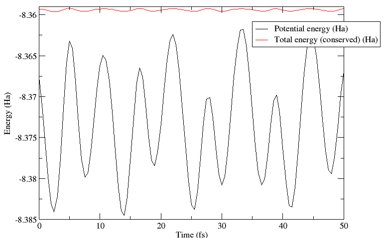
where the default timestep (0.5fs) is necessary for simulations
involving light atoms like hydrogen. The file md.stats contains
details of the simulation, while the trajectory is output to
trajectory.xsf which can be read by VMD among other programs. In
this simulation, the conserved quantity is the total energy (the sum
of ionic kinetic energy and potential energy of the system) which is
maintained to better than 0.1mHa in this instance. More importantly,
the variation in this quantity is much smaller than the variation in
the potential energy. This can be seen in the plot below.
Go to top.
Tutorials
We recommend that you work through, in order, the tutorials included
in the distribution in the tutorials/ directory
to become familiar with the modes of operation of the code.
NOTE In the initial pre-release of CONQUEST (January 2020) we have not included the tutorials; they will be added over the coming months.
Go to top.
Where next?
While the tutorials have covered the basic operations of Conquest, there are many more subtle questions and issues, which are given in the User Guide.
Go to top.